Research article
Volatility and Asymmetric Shocks in Bangladesh’s Stock Market: An EGARCH Analysis of the DSEX
Evidence from Daily DSEX Returns, January 2013–September 2026
TradeBiz Economy
25 September 2026
Abstract
This study examines volatility persistence and asymmetric responses to market shocks in the Dhaka Stock Exchange Broad Index (DSEX). It uses 3,125 daily closing-index observations from 31 January 2013 to 21 September 2026, producing 3,124 continuously compounded daily returns. Preliminary tests show that returns are stationary, non-normal and strongly affected by conditional heteroskedasticity. An AR(5) mean equation is combined with GARCH(1,1), EGARCH(1,1) and GJR-GARCH(1,1) variance specifications under standardized Student-t errors. EGARCH(1,1) provides the best fit, with the lowest Akaike and Bayesian information criteria. Its negative asymmetry parameter is statistically significant, indicating a stronger conditional-volatility response to adverse shocks than to favourable shocks of equal magnitude. The persistence coefficient is high, showing that shocks dissipate gradually. Post-estimation diagnostics find no significant remaining ARCH effects in squared standardized residuals. The results support the use of asymmetric, heavy-tailed volatility models for risk monitoring in Bangladesh, while also showing why volatility forecasts should not be interpreted as predictions of market direction.
Keywords: DSEX; stock-market volatility; EGARCH; asymmetric shocks; leverage effect; Student-t distribution; Bangladesh
List of Abbreviations
| Abbreviation | Meaning |
|---|---|
| ADF | Augmented Dickey-Fuller |
| AIC | Akaike Information Criterion |
| ARCH | Autoregressive Conditional Heteroskedasticity |
| BIC | Bayesian Information Criterion |
| DSE | Dhaka Stock Exchange |
| DSEX | Dhaka Stock Exchange Broad Index |
| EGARCH | Exponential Generalized Autoregressive Conditional Heteroskedasticity |
| GARCH | Generalized Autoregressive Conditional Heteroskedasticity |
| GJR-GARCH | Glosten-Jagannathan-Runkle GARCH |
| JB | Jarque-Bera |
| Q² | Ljung-Box statistic applied to squared residuals |
1 Introduction
Stock-market volatility matters because it affects investment decisions, financing conditions, portfolio risk, market surveillance and confidence in the capital market. A rise in an index and a rise in volatility are not the same phenomenon. The index measures the level of market prices, whereas volatility measures the size and variability of returns. A market may rise while remaining highly volatile, or fall gradually with comparatively modest volatility.
Daily financial returns rarely satisfy the assumption of constant variance. Large changes tend to be followed by large changes and quiet periods tend to be followed by quiet periods, a pattern known as volatility clustering. Return distributions also commonly have heavy tails, meaning that extreme movements occur more frequently than a normal distribution would predict. These features motivated the ARCH model of Engle (1982), the GARCH extension of Bollerslev (1986), and subsequent asymmetric models.
Asymmetry is particularly important. In many equity markets, unfavourable information produces a larger increase in volatility than favourable information of the same magnitude. Nelson’s (1991) EGARCH formulation captures this sign effect while modelling the logarithm of conditional variance, thereby ensuring a positive variance without imposing the non-negativity restrictions required by linear GARCH models.
This study asks three questions. First, do DSEX returns display conditional heteroskedasticity and volatility clustering? Second, does an asymmetric specification fit the data better than symmetric GARCH? Third, what do the estimated magnitude, asymmetry and persistence parameters imply for market-risk analysis in Bangladesh?
2 Review of Empirical and Policy Literature
The international literature establishes several relevant propositions. Engle (1982) showed that conditional variance can depend on past squared innovations. Bollerslev (1986) extended this approach by allowing conditional variance to depend on both past shocks and its own lagged values. Nelson (1991) introduced EGARCH to model the logarithm of conditional variance and permit asymmetric effects. Alberg, Shalit and Yosef (2008) found that asymmetric GARCH specifications can perform well when modelling equity volatility. The literature also shows that distributional choice matters: Student-t innovations often provide a more realistic representation of financial returns because normal errors understate tail risk.
Bangladesh-focused studies consistently report non-normal returns, volatility clustering and persistent conditional variance. Basher, Hassan and Islam (2007) examined time-varying volatility and the effects of institutional arrangements in the Bangladesh equity market. Rahman and Moazzem (2011) discussed DSE volatility alongside the role of regulators. Aziz and Uddin (2015) applied GARCH models to DSE returns and identified unusually volatile periods around the 2010–2011 market episode.
Siddikee and Begum (2016) used DGEN returns from 2002 to 2013 and found abnormal volatility from 2009 to 2012, with 2011 showing the highest estimated daily volatility. Huq, Karim and Ali (2017) compared GARCH, EGARCH, TGARCH and PARCH models for DSE and CSE data. They found stationary but leptokurtic returns, significant ARCH effects, volatility persistence and leverage effects. Bhowmik et al. (2017) likewise reported that volatility characteristics changed across pre-crisis, crisis and post-crisis periods, supporting the use of flexible GARCH-family models.
More recent work has refined the interpretation of asymmetric news effects. Bose and Rahman (2022) directly examined whether news effects are necessarily asymmetric in the Bangladesh market, emphasising that the sign and statistical significance of news effects should be tested rather than assumed. That caution is followed here: model choice is based on the supplied data, information criteria and residual diagnostics, not on a prior presumption that asymmetry must exist.
The present study extends much of the earlier Bangladesh literature in three respects. It uses the DSEX broad index over a substantially longer period ending in September 2026; it compares symmetric and asymmetric specifications under heavy-tailed errors; and it reports equations, variable definitions and diagnostic tests in a form intended to be accessible to students, practitioners and policy readers.
3 Rationale and Objectives
The rationale is practical as well as empirical. Bangladesh’s capital market has experienced periods of rapid movement, regulatory intervention, changing liquidity and major domestic and external disturbances. A model that assumes constant risk cannot describe these dynamics adequately. The purpose is therefore to estimate conditional volatility, test whether negative and positive shocks have different effects, and identify a parsimonious model suitable for monitoring market risk.
The study does not attempt to produce a mechanical trading rule. Its objective is to explain and forecast the conditional variance of returns. Directional price forecasting, causal identification of particular policy events and company-level valuation remain outside its scope.
4 Data and Methodology
4.1 Data and return construction
The dataset contains 3,125 daily DSEX observations from 31 January 2013 to 21 September 2026. The closing-index series is complete. The source file also contains opening, high and low values; however, the volume field is blank and is excluded. After ordering the observations chronologically, 3,124 daily logarithmic returns are calculated as follows:

Here, r_t denotes the continuously compounded daily return in percentage terms, P_t is the closing DSEX value on trading day t, and ln denotes the natural logarithm.
4.2 Preliminary tests
The analysis begins with descriptive statistics, the ADF test for stationarity, the Jarque-Bera test for normality, Ljung-Box tests for serial dependence in returns and squared returns, and an ARCH-LM test. Strong dependence in squared returns and a significant ARCH-LM statistic provide the empirical basis for estimating conditional-variance models.
4.3 Mean equation
Autoregressive orders from zero to five are compared. BIC favours a shorter AR(1), while AIC favours AR(5). Because the AR(1) specification leaves significant serial correlation in standardized residuals, the AR(5) equation is retained for the final volatility comparison:

The constant is c, phi_i denotes the autoregressive coefficients, and epsilon_t is the return innovation.
4.4 Conditional-variance models
Three models are estimated: symmetric GARCH(1,1), EGARCH(1,1), and GJR-GARCH(1,1). The principal EGARCH variance equation is:

 In the last expression, t_nu
denotes the unit-variance standardized Student-t distribution, rather
than the unscaled Student-t distribution.
Here, h_t is the conditional variance of the return innovation epsilon_t; its square root is conditional standard deviation. The standardized innovation is z_t = epsilon_t / sqrt(h_t), with zero mean and unit variance. E|z_t| is its expected absolute value. Omega is the log-variance constant; alpha measures the magnitude effect of a shock relative to E|z_t|; beta measures persistence; and gamma measures the sign effect. A negative gamma implies a larger fitted log-variance response to a negative than to an equally sized positive standardized shock. The innovation follows a unit-variance standardized Student-t distribution with nu degrees of freedom (nu > 2), allowing heavy tails.
4.5 Model selection and diagnostics
Maximum likelihood estimation is used. Robust (sandwich) standard errors are used for coefficient inference. The AR(5) model has 3,119 effective return observations after five lags; the underlying return series contains 3,124 observations. Competing models are ranked using AIC and BIC, where lower values indicate better relative fit after penalising model complexity. Adequacy is then assessed through Ljung-Box tests on standardized and squared standardized residuals and a residual ARCH-LM test. The primary concern for the variance equation is whether significant dependence remains in squared standardized residuals.
5 Empirical Results
5.1 Behaviour of the index and returns
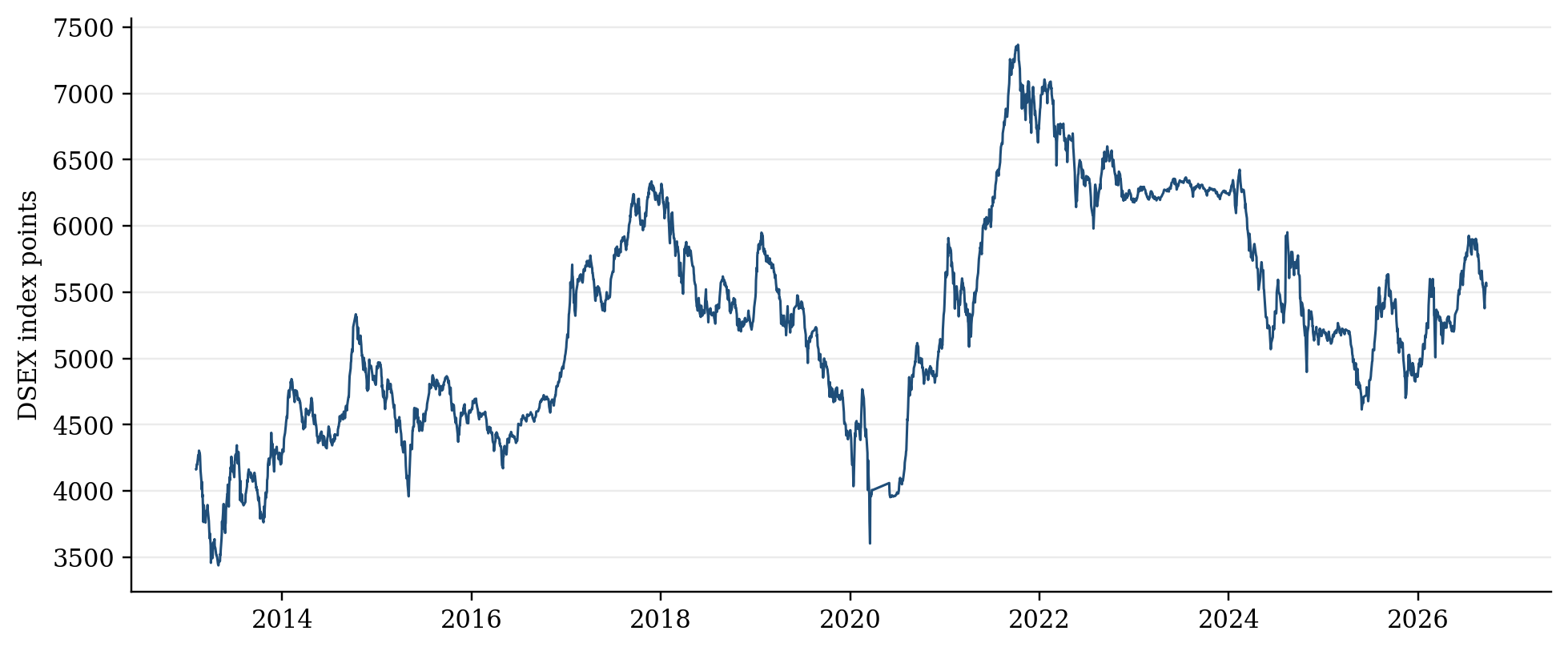
Figure 1 Daily DSEX closing index, January 2013–September 2026
The index level shows several distinct cycles rather than a smooth trend. Periods of advance are interrupted by substantial corrections, most visibly around the sharp market disturbance in 2020 and subsequent phases of recovery and renewed weakness. These level movements do not by themselves measure volatility, but they provide the market context for the return series.
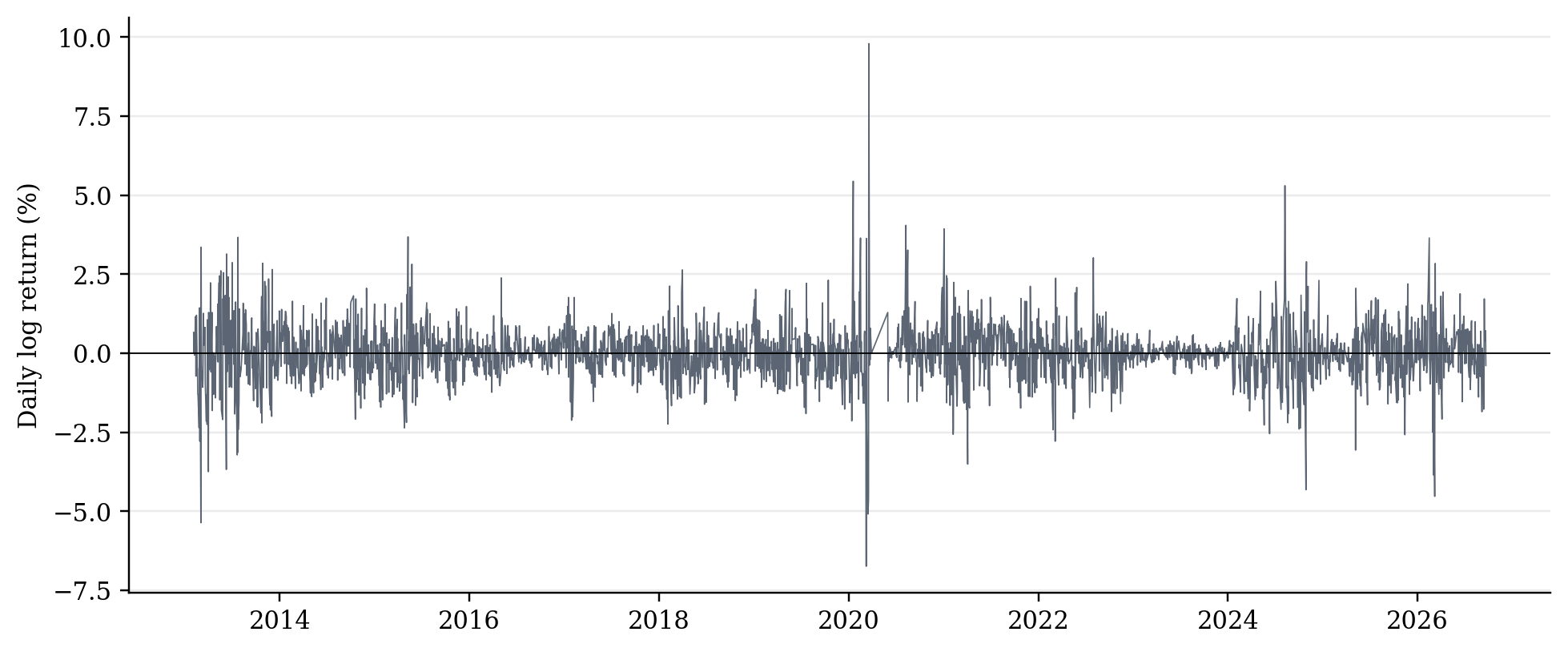
Figure 2 Daily logarithmic DSEX returns
Figure 2 shows clear volatility clustering. Large positive and negative returns occur in groups, and the amplitude of returns changes materially over time. This visual pattern is consistent with the formal ARCH tests.
5.2 Descriptive statistics and preliminary tests
Table 1 Descriptive statistics for daily DSEX returns
| Measure | Result |
|---|---|
| Return observations | 3,124 |
| Mean daily return | 0.0094% |
| Standard deviation | 0.8707% |
| Minimum daily return | -6.7371% |
| Maximum daily return | 9.7984% |
| Skewness | 0.3231 |
| Excess kurtosis | 9.9811 |
Table 1 reports these results. The mean daily return is close to zero relative to its standard deviation. Excess kurtosis is approximately 9.98, confirming a sharply peaked and heavy-tailed distribution. The maximum and minimum returns also show that extreme daily movements are economically material.
Table 2 Preliminary stationarity, normality and ARCH diagnostics
| Diagnostic test | Statistic or p-value | Decision |
|---|---|---|
| ADF test | Statistic = -20.2371 | Returns are stationary |
| Jarque-Bera | p < 0.001 | Reject normality |
| Ljung-Box Q(10), returns | p < 0.001 | Serial correlation is present |
| Ljung-Box Q²(10), squared returns | p < 0.001 | Strong volatility clustering |
| ARCH-LM(10) | Statistic = 486.7521; p < 0.001 | Conditional heteroskedasticity is present |
Table 2 reports these results. The ADF statistic is far below the approximate 1 per cent critical value, supporting stationarity of returns. Normality is decisively rejected. More importantly, squared returns display strong serial dependence and the ARCH-LM test is highly significant. A constant-variance model is therefore inappropriate.
5.3 Comparison of volatility models
Table 3 Comparison of conditional-variance models
| Model | Log likelihood | AIC | BIC | Persistence | Residual ARCH-LM p |
|---|---|---|---|---|---|
| GARCH | -3287.75 | 6595.51 | 6655.96 | 0.9950 | 0.2297 |
| EGARCH | -3247.76 | 6517.53 | 6584.03 | 0.9595 | 0.1927 |
| GJR-GARCH | -3287.75 | 6597.51 | 6664.01 | 0.9950 | 0.2297 |
Table 3 reports these results. EGARCH produces the highest log likelihood and the lowest AIC and BIC. Its advantage is substantial rather than marginal: the EGARCH BIC is about 72 points below that of GARCH and 80 points below GJR-GARCH. The model is therefore selected as the preferred specification.
5.4 EGARCH estimates and interpretation
Table 4 AR(5)–EGARCH(1,1) parameter estimates
| Parameter | Estimate | Interpretation |
|---|---|---|
| Mean constant | -0.0060 | Conditional mean intercept |
| AR(1) | 0.1828 | First-order return dependence |
| AR(2) | -0.0358 | Second-order return dependence |
| AR(3) | 0.0703 | Third-order return dependence |
| AR(4) | 0.0534 | Fourth-order return dependence |
| AR(5) | 0.0175 | Fifth-order return dependence |
| omega | -0.0180 | Log-variance constant |
| alpha | 0.3739 | Magnitude effect of new shocks |
| gamma | -0.0780 | Negative asymmetry; robust SE 0.0144; z -5.43; p 5.68e-08 |
| beta | 0.9596 | High volatility persistence |
| nu | 8.6249 | Student-t degrees of freedom; heavy tails |
Table 4 reports these results. The independently re-estimated asymmetry coefficient is gamma = -0.0780, with robust standard error 0.0144, z = -5.43 and p = 5.68e-08. The two-sided 95 per cent robust confidence interval is [-0.1062, -0.0498]. The coefficient is significantly negative, implying a larger fitted volatility response to negative than to equally sized positive innovations within the stated EGARCH parameterisation.
The persistence coefficient beta = 0.9596 is high but below unity. A volatility shock therefore has a long memory in the practical sense that its effect decays gradually. This does not mean volatility remains permanently at an elevated level; it means that a large disturbance can influence estimated risk over many subsequent trading sessions.
The magnitude parameter alpha = 0.3739 indicates a sizeable reaction to the absolute size of standardized shocks. The Student-t degrees-of-freedom estimate of about 8.62 confirms heavier tails than the normal distribution. This choice reduces the risk that a few extreme observations distort the variance estimates or are treated as virtually impossible events.
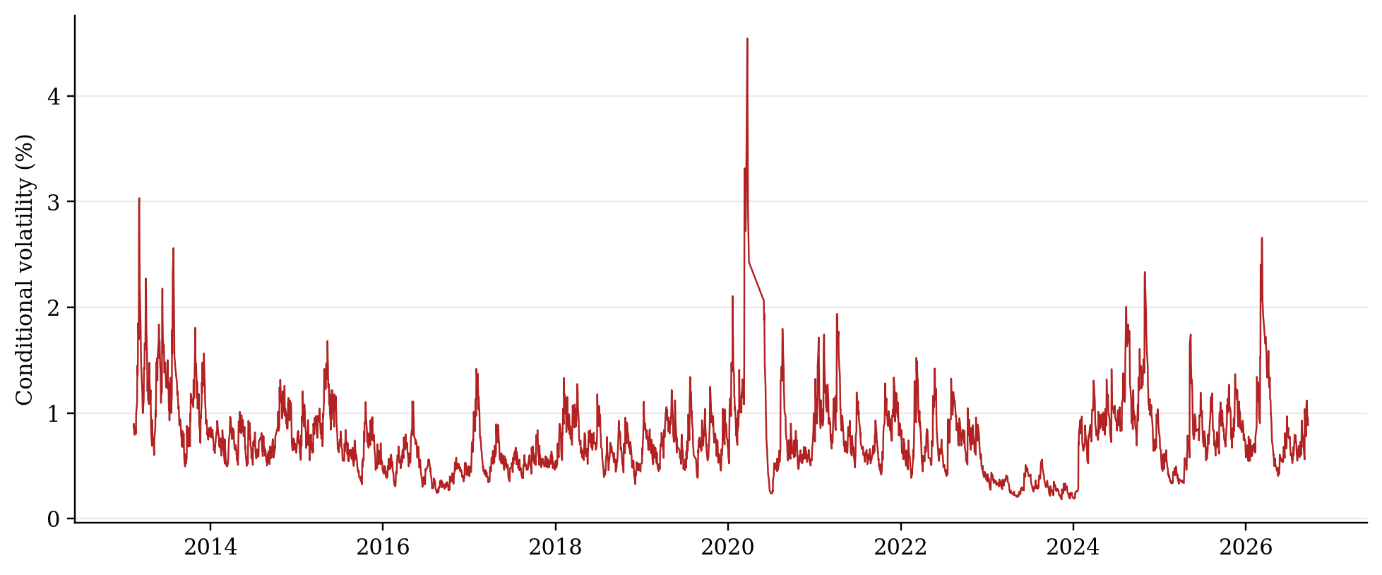
Figure 3 Estimated conditional volatility from the AR(5)–EGARCH(1,1) Student-t model
Conditional volatility varies considerably through the sample. The largest spike occurs around the exceptional market disturbance in 2020. Other elevated episodes appear at the beginning of the sample and again toward the end. The model therefore distinguishes periods of relatively subdued risk from periods when market uncertainty rises sharply.
5.5 Residual diagnostics
Table 5 Residual diagnostics for the selected EGARCH model
| Diagnostic | p-value | Assessment |
|---|---|---|
| Ljung-Box Q(10), standardized residuals | 0.0319 | Some remaining short-run mean dependence |
| Ljung-Box Q(20), standardized residuals | 0.0499 | Borderline at the 5% level |
| Ljung-Box Q²(10), squared standardized residuals | 0.2205 | No significant remaining volatility dependence |
| Ljung-Box Q²(20), squared standardized residuals | 0.1258 | No significant remaining volatility dependence |
| ARCH-LM(10) | 0.1927 | No significant remaining ARCH effect |
Table 5 reports these results. The squared-residual and ARCH-LM diagnostics are satisfactory for the variance equation. The model captures the volatility clustering that motivated the analysis. Some short-run autocorrelation remains in standardized residuals, so the mean specification could be refined in future forecasting exercises. This limitation does not overturn the reported in-sample model ranking or the robust significance test for the asymmetry coefficient.
6 Discussion
The results align with the main pattern reported in earlier Bangladesh studies: returns are non-normal, conditional variance changes over time, volatility is persistent and asymmetric models can improve in-sample fit over symmetric GARCH. The longer sample used here indicates that these features are not confined to the 2010–2011 market episode. They remain visible across later regulatory, political, economic and pandemic-related disturbances.
The comparison between EGARCH and GJR-GARCH is instructive. The estimated GJR asymmetry term is close to zero in the present optimisation, whereas EGARCH achieves a much better likelihood and information criteria. This suggests that the logarithmic response form in EGARCH describes the data more effectively than the particular threshold form imposed by GJR-GARCH. It does not establish that every negative return causes volatility or that all bad news has the same effect.
The negative gamma should be interpreted as conditional asymmetry, not a causal estimate of any particular announcement. Establishing why a specific episode raised volatility would require event indicators, trading-volume and liquidity measures, macroeconomic variables, regulatory dates or higher-frequency data. The present model answers a narrower but useful question: given past returns and variance, does the sign of the latest innovation help explain current conditional volatility? The estimated coefficient is negative and statistically significant within the selected specification.
7 Implications and Recommendations
7.1 For investors and market professionals
Risk estimates should be allowed to change through time. A fixed historical standard deviation can understate risk after a shock and overstate it during calm periods. Conditional-volatility measures can support portfolio limits, stress testing, margin policies and scenario analysis. Because Student-t tails are material, risk systems should not rely solely on normal-distribution thresholds. Volatility forecasts should nevertheless remain separate from directional investment decisions.
7.2 For market institutions and regulators
Market surveillance can monitor volatility persistence alongside index movements, turnover, liquidity and concentration. A sharp increase in estimated conditional volatility may justify closer observation of order imbalances, settlement pressure and information dissemination, but it should not automatically trigger intervention. Circuit breakers and other stabilisation measures should be evaluated using event-based research that distinguishes temporary disruption from normal price discovery.
7.3 For disclosure and investor education
Investor communication should distinguish market loss, volatility and liquidity risk. A volatile market is not necessarily falling every day, and a rising market is not necessarily low-risk. Public educational materials can explain that the estimated model suggests that negative shocks may have larger effects on uncertainty and that risk can remain elevated after the initial event has passed.
7.4 For future analytical work
A regular monitoring framework could re-estimate the model as new observations arrive and compare one-day and multi-day volatility forecasts with realised outcomes. Forecast evaluation should use an out-of-sample period and loss functions designed for volatility. Extensions may incorporate trading volume, exchange-rate changes, interest rates, inflation surprises, policy announcements and structural-break indicators.
8 Limitations
The analysis has five main limitations. First, it uses the broad market index and does not reveal differences across sectors or individual securities. Second, the source file contains no usable volume observations, so liquidity cannot be modelled. Third, the analysis focuses on conditional volatility rather than causal identification of events. Fourth, the model comparison is in-sample; formal forecasting claims require out-of-sample evaluation. Fifth, remaining autocorrelation in standardized residuals indicates scope to refine the mean equation, consider calendar effects or allow structural breaks.
9 Conclusion
DSEX returns from February 2013 to September 2026 are stationary, heavy-tailed and characterised by strong volatility clustering. These properties justify a conditional heteroskedasticity framework. Among the estimated alternatives, the AR(5)–EGARCH(1,1) model with standardized Student-t errors provides the best fit by both AIC and BIC. The statistically significant negative asymmetry coefficient indicates a larger fitted volatility effect from adverse shocks than from favourable shocks of comparable size. The high persistence coefficient indicates that elevated risk dissipates slowly.
The model successfully removes the original ARCH dependence from squared standardized residuals and provides a useful description of time-varying market risk. Its proper use is therefore risk measurement and volatility forecasting—not automatic prediction of whether the DSEX will rise or fall. For investors, market institutions and policy analysts, the broader lesson is that estimated risk is dynamic, asymmetric and sensitive to extreme observations. Monitoring systems should be designed accordingly.
References
Alberg, D., Shalit, H. and Yosef, R. (2008) ‘Estimating stock market volatility using asymmetric GARCH models’, Applied Financial Economics, 18(15), pp. 1201–1208.
Aziz, M.S.I. and Uddin, M.N. (2015) ‘Volatility estimation in the Dhaka Stock Exchange returns by GARCH models’, Asian Business Review, 4(1), pp. 41–49.
Basher, S.A., Hassan, M.K. and Islam, A.M. (2007) ‘Time-varying volatility and equity returns in Bangladesh stock market’, Applied Financial Economics, 17(17), pp. 1393–1407. doi: 10.1080/09603100600771034.
Bhowmik, R., Wu, C., Kumar, J.R. and Wang, S. (2017) ‘A study on the volatility of the Bangladesh stock market—Based on GARCH type models’, Journal of Systems Science and Information, 5(3), pp. 193–215. doi: 10.21078/JSSI-2017-193-23.
Bollerslev, T. (1986) ‘Generalized autoregressive conditional heteroskedasticity’, Journal of Econometrics, 31(3), pp. 307–327.
Bose, S. and Rahman, H. (2022) ‘Are news effects necessarily asymmetric? Evidence from Bangladesh stock market’, SAGE Open, 12(4), pp. 1–17. doi: 10.1177/21582440221127157.
Engle, R.F. (1982) ‘Autoregressive conditional heteroscedasticity with estimates of the variance of United Kingdom inflation’, Econometrica, 50(4), pp. 987–1007.
Huq, M.M., Karim, M.M. and Ali, M.A. (2017) ‘Modeling and forecasting of return volatility in Bangladeshi stock markets under GARCH framework’, International Journal of Statistical Sciences, 16, pp. 49–66.
Nelson, D.B. (1991) ‘Conditional heteroskedasticity in asset returns: A new approach’, Econometrica, 59(2), pp. 347–370.
Rahman, M.T. and Moazzem, K.G. (2011) ‘Capital market of Bangladesh: Volatility in the Dhaka Stock Exchange and role of regulators’, International Journal of Business and Management, 6(7), pp. 86–93.
Siddikee, M.N. and Begum, N.N. (2016) ‘Volatility of Dhaka Stock Exchange’, International Journal of Economics and Finance, 8(5), pp. 220–229.
Back to top ↑